Flash Attention

Flash Attention 优势

Fast（with IO-Awareness）

计算快。在 Flash Attention 之前，也出现过一些加速 Transformer 计算的方法，这些方法的着眼点是“减少计算量 FLOPs”，例如用一个稀疏 attention 做近似计算。

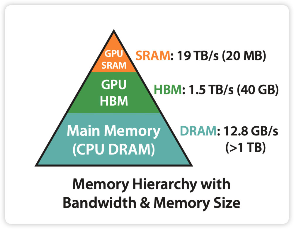
但是 Flash attention 就不一样了，它并没有减少总的计算量，因为它发现：计算慢的卡点不在运算能力，而是在读写速度上。 所以它通过降低对显存 HBM 的访问次数来加快整体运算速度，这种方法又被称为IO-Awareness。在后文中，我们会详细来看 Flash Attention 是如何通过分块计算（tiling） 和 核函数融合（kernel fusion） 来降低对显存的访问。

Memory Efficicent

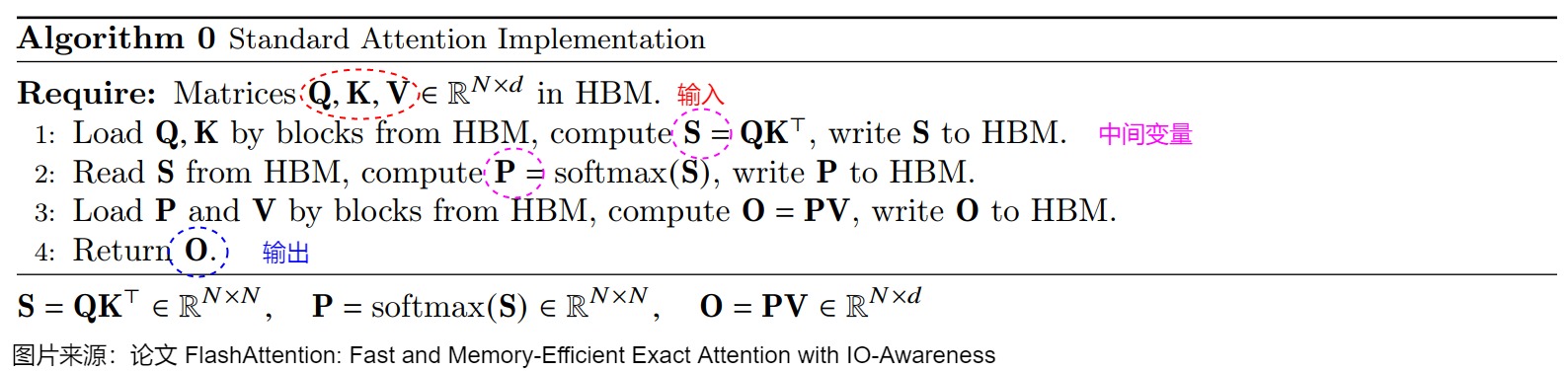
节省显存。在标准 attention 场景中，forward 时我们会计算并保存 $N*N$ 大小的注意力矩阵；在 backward 时我们又会读取它做梯度计算，这就给硬件造成了 $O(N^2)$ 的存储压力。在 Flash Attention 中，则巧妙避开了这点，使得存储压力降至 $O (N)$。在后文中我们会详细看这个 trick。

Exact Attention

精准注意力。之前的办法会采用类似于 稀疏 attention 的方法做近似。这样虽然能减少计算量，但算出来的结果并不完全等同于标准 attention 下的结果。但是 Flash Attention 却做到了完全等同于标准 attention 的实现方式。

从 Online Softmax 到 FlashAttention

对于经典的 Multi-head Attention，计算方式如下所示（为了表示简单，这里省去了 scale factor） $$ O = Attention(Q,K,V) = softmax(QK^T) V $$

当 sequence length 增加时，模型计算量和存储占用复杂度随着序列长度呈二次方增长。内存占用 $N^2$ 的关键，就在于 Attention Score $S = Q^KT$ 的计算，当 sequence length 增加时，显存占用以 $O(N^2)$ 比例增加。

Safe Softmax：3-pass

Softmax 计算公式如下所示： $$ \text{softmax}({x_1, \dots, x_N}) = \left{ \frac{e^{x_i}}{\sum_{j=1}^N e^{x_j}} \right}{i=1}^N $$ 考虑到 $x_i$ 可能非常大，那么 $e^{x_i}$ 会很容易 overflow，比如 float16 最大支持 65536，那么如果 $x \geqslant 11$, $e^x$ 会超过 float16 的表示范围。为了计算更加稳定，会用以下 saft softmax 来计算，其中 $m = \max{j=1}^N (x_j)$，这样每个 $x_i - m \leqslant 0$ $$ \frac{e^{x_i}}{\sum_{j=1}^N e^{x_j}} = \frac{e^{x_i - m}}{\sum_{j=1}^N e^{x_j - m}} $$

这个时候对应的 3-pass 计算 softmax：

• Pass 1: 遍历 N 次计算 $x_i$ 的最大值 $m$
• Pass 2: 遍历 N 次分别计算指数，累积求和得到 softmax 分母
• Pass 3: 遍历 N 次分别计算得到 $x_i$ 的 softmax 值

对应到 Attention 计算中，$x$ 就是将计算得到的 $S=QK^T$，对应的 shape 是 $(N, N)$ 。考虑到 GPU 的 SRAM 一般比较小，$S$ 由于需要 $O(N^2)$ 的显存无法放在 SRAM 中，比如 $N=4k$ 的时候，至少需要 $4k * 4k * 2 = 32M$ 字节的空间存储 $S$ 状态。而对于 GPU SRAM 一般比较小，随着 sequence length 增加，$S$ 状态一般是存储不下的。

因此，这种状态下，只能每次循环中去 load 一部分 Q，K 到 SRAM，计算得到 $x$。按照 3 Pass 计算方法，我们要将 $x$ 从 Global Memory 取 3 次到 SRAM。

对应的代码实现如下所示：

 1
 2
 3
 4
 5
 6
 7
 8
 9
10
11

def safe_softmax_three_pass(x):
    """Safe Softmax implementation using three passes to avoid overflow."""
    # Pass 1: Compute the maximum value for numerical stability
    m = torch.max(x)
    
    # Pass 2: Compute the exponentials
    exp_x = torch.exp(x - m)
    
    # Pass 3: Compute the sum and normalize
    sum_exp_x = torch.sum(exp_x)
    return exp_x / sum_exp_x

Online Softmax: 2-pass

如果能够把上面的 7/8/9 三个公式合成一个，那么可以将访问 Global Memory 的次数从 3 次降低到 1 次。但是因为公式 8 依赖于公式 7 的 $m_N$，所以不能合并。

令 $d’i := \sum{j=1}^i e^{x_j - m_i}$ 作为原始公式 $d_i := \sum_{j=1}^i e^{x_j - m_N}$ 的替代，来移除对于 $N$ 的依赖。可以看到这两个公式的第 $N$ 个值是相等的: $d_N = d’_N$ ，因此，只要我们计算出了 $d’_N$ ，就可以用它来代替公式 9 的 $d_N$。

关于 $d’i$ 和 $d’{i-1}$ 之间的递推公式： $$ \begin{align*} d’i &= \sum{j=1}^i e^{x_j - m_i} \ &= \left( \sum_{j=1}^{i-1} e^{x_j - m_i} \right) + e^{x_i - m_i} \ &= \left( \sum_{j=1}^{i-1} e^{x_j - m_{i-1}} \right) e^{m_{i-1} - m_i} + e^{x_i - m_i} \ &= d’{i-1} e^{m{i-1} - m_i} + e^{x_i - m_i} \end{align*} $$

这里的递推公式只依赖于 $m_i$ 和 $m_{i-1}$, 因此可以在一个 loop 里一起计算 $m_j$ and $d’_j$

对应的代码如下所示：

 1
 2
 3
 4
 5
 6
 7
 8
 9
10
11
12

def online_softmax(x):
    """Online Softmax implementation using two passes for efficiency."""
    # Pass 1: Compute maximum and sum of exponentials in one traversal
    m = float('-inf')  # Current maximum
    s = 0.0            # Sum of exponentials
    for xi in x:
        m_old = m
        m = max(m, float(xi))
        s = s * torch.exp(torch.tensor(m_old - m)) + torch.exp(xi - m)
    
    # Pass 2: Normalize
    return torch.tensor([torch.exp(xi - m) / s for xi in x])

Flash Attention: 1-pass

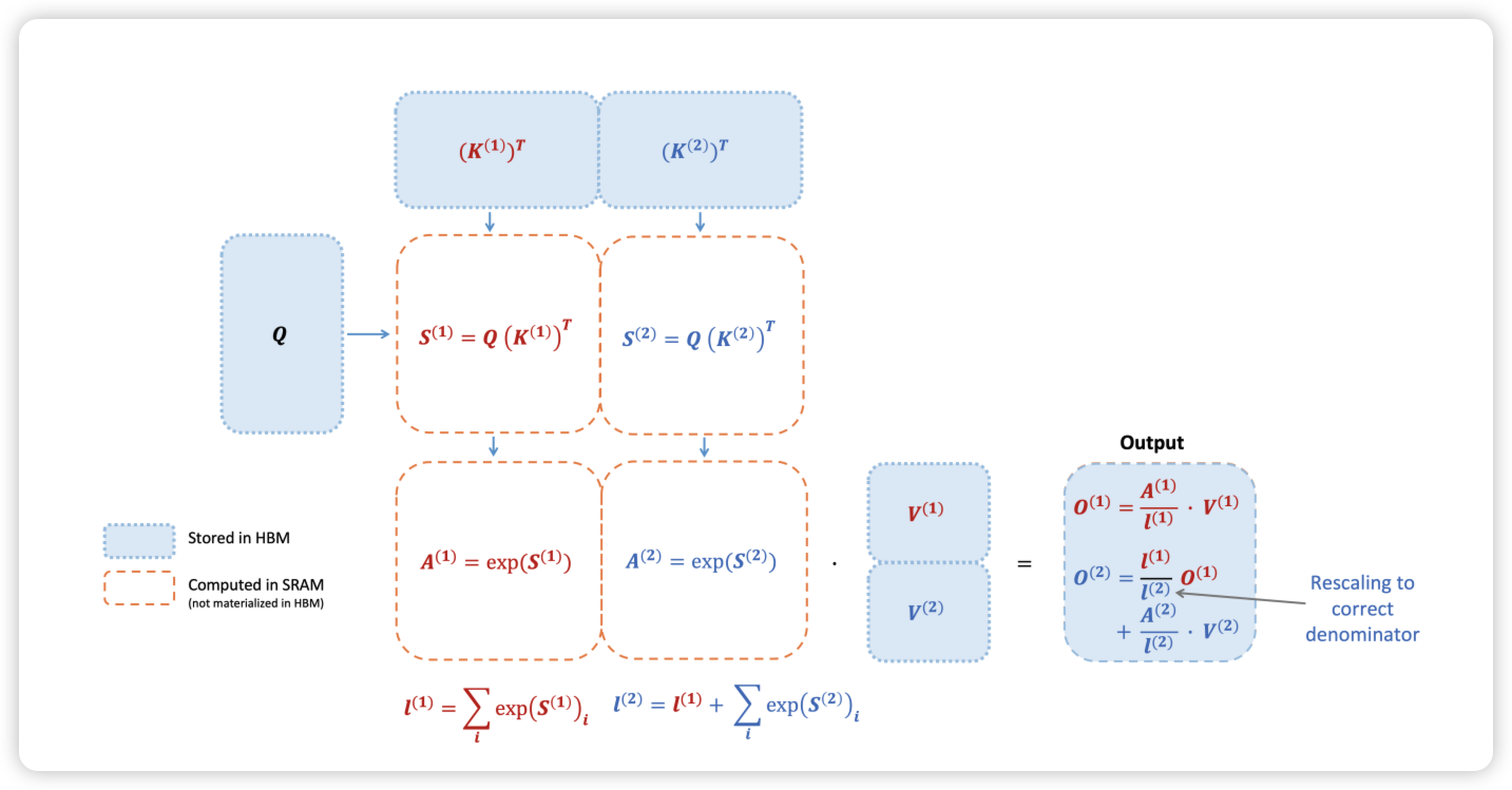
可以看到，online softmax 将遍历次数降低到 2 pass，那么是否还可以降低到 1 pass 呢？可以的是，对于 softmax 是不可以的。不过，对于 Attention，最终目标不是计算出 Attention $P=softmax(S)$，而是计算出 $O=PV$。对于 O 是否可以实现 1 pass 计算出来呢？

下面尝试计算第 $k$ 个 token 的 score，其中 $Q, K, V \in R^{N\times d}$，因此对应于 $Q$ 中的第 $k$ 行。而且每个 token 的 score 计算都是独立的，因此可以代表所有 token 的计算方法：

我们将公式 11 中的 $a_i$ 代入到公式 12，得到：

$$ \boldsymbol{o}i := \sum{j=1}^i \left( \frac{e^{x_j - m_N}}{d_N’} V[j,:] \right) \tag{13} $$

这个公式仍然依赖于 $m_N$ 和 $d_N$，同样适用替代目标 $\boldsymbol{o}’$，

$$

\boldsymbol{o}’i := \left( \sum{j=1}^i \frac{e^{x_j - m_i}}{d’_i} V[j,:] \right)

$$

同样有，对于 $\boldsymbol{o}$ and $\boldsymbol{o}’$ 第 $N$ 项是相同的: $\boldsymbol{o}’_N = \boldsymbol{o}_N$

我们可以得到 $\boldsymbol{o}’i$ and $\boldsymbol{o}’{i-1}$ 之间的递推公式：

$$

\begin{align*}

\boldsymbol{o}’i &= \sum{j=1}^i \frac{e^{x_j - m_i}}{d’_i} V[j,:] \

&= \left( \sum_{j=1}^{i-1} \frac{e^{x_j - m_i}}{d’_i} V[j,:] \right) + \frac{e^{x_i - m_i}}{d’_i} V[i,:] \

&= \left( \sum_{j=1}^{i-1} \frac{e^{x_j - m_{i-1}}}{d’{i-1}} \frac{e^{x_j - m_i}}{e^{x_j - m{i-1}}} \frac{d’_{i-1}}{d’_i} V[j,:] \right) + \frac{e^{x_i - m_i}}{d’_i} V[i,:] \

&= \left( \sum_{j=1}^{i-1} \frac{e^{x_j - m_{i-1}}}{d’{i-1}} V[j,:] \right) \frac{d’{i-1} e^{m_{i-1} - m_i}}{d’_i} + \frac{e^{x_i - m_i}}{d’_i} V[i,:] \

&= \boldsymbol{o}’{i-1} \frac{d’{i-1} e^{m_{i-1} - m_i}}{d’_i} + \frac{e^{x_i - m_i}}{d’_i} V[i,:]

\end{align*}

$$

$\boldsymbol{o}’i$ and $\boldsymbol{o}’{i-1}$ 只依赖于 $d’i$, $d’{i-1}$, $m_i$, $m_{i-1}$ and $x_i$，因此，我们就可以实现 1 pass 计算 flash attention

对应代码如下：

 1
 2
 3
 4
 5
 6
 7
 8
 9
10
11
12
13
14
15
16
17
18
19
20
21
22
23
24
25
26
27
28
29
30
31
32
33
34
35
36
37
38
39
40
41
42
43
44

def flash_attention_v1(Q, K, V):
    """
    FlashAttention V1 implementation with single-pass computation.
    Fuses Softmax(QK^T)V into one loop without storing S or P.
    
    Args:
        Q, K, V: Query, Key, Value matrices of shape (seq_len, head_dim)
    Returns:
        Output of attention: (seq_len, head_dim)
    """
    seq_len, head_dim = Q.shape
    scale = 1.0 / (head_dim ** 0.5)  # Scaling factor 1/sqrt(d)
    
    # Initialize output and running statistics
    O = torch.zeros_like(Q)  # Output
    l = torch.zeros(seq_len, dtype=torch.float32, device=Q.device)  # Sum of exponentials (d_i')
    m = torch.full((seq_len,), float('-inf'), device=Q.device)  # Max values (m_i)
    
    # Single pass over sequence length
    for i in range(seq_len):
        # Compute Q[i] * K^T for row i
        S_i = torch.matmul(Q[i:i+1], K.transpose(-1, -2)) * scale  # Shape: (1, seq_len)
        
        # Online Softmax for row i
        m_i = torch.max(S_i)  # Current max (m_i)
        m_old = m[i]  # Previous max (m_{i-1})
        m_new = torch.maximum(m_old, m_i)  # Update max
        l_old = l[i]  # Previous sum (d_{i-1}')
        
        # Update sum of exponentials (d_i')
        exp_diff = torch.exp(m_old - m_new)
        exp_S = torch.exp(S_i - m_new)
        l_new = l_old * exp_diff + torch.sum(exp_S)
        
        # Update output: O[i] = O[i] * exp(m_old - m_new) + exp(S_i - m_new) * V
        O[i] = O[i] * exp_diff + torch.matmul(exp_S / l_new, V)
        
        # Update statistics
        m[i] = m_new
        l[i] = l_new
    
    # Final normalization
    O = O / l.unsqueeze(-1)
    return O

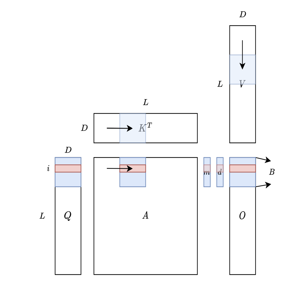
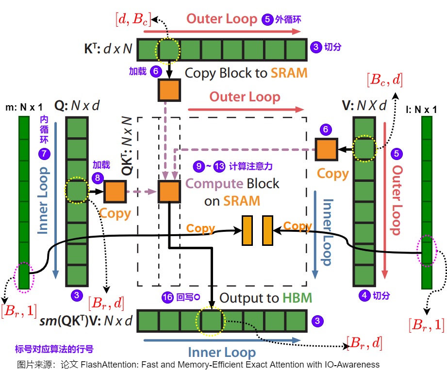
Flash Attention: Tiling

代码如下：

 1
 2
 3
 4
 5
 6
 7
 8
 9
10
11
12
13
14
15
16
17
18
19
20
21
22
23
24
25
26
27
28
29
30
31
32
33
34
35
36
37
38
39
40
41
42
43
44
45
46
47
48
49
50
51
52
53
54
55
56
57
58
59
60
61
62
63

def flash_attention_v1_tiling(Q, K, V, tile_size=128):
    """
    FlashAttention V1 implementation with tiling to leverage SRAM.
    Fuses Softmax(QK^T)V into one kernel with tiled computation.
    
    Args:
        Q, K, V: Query, Key, Value matrices of shape (seq_len, head_dim)
        tile_size: Size of each tile for tiling computation
    Returns:
        Output of attention: (seq_len, head_dim)
    """
    seq_len, head_dim = Q.shape
    d = head_dim  # Head dimension for scaling
    scale = 1.0 / (d ** 0.5)
    
    # Initialize output and normalization statistics
    O = torch.zeros_like(Q)  # Output
    l = torch.zeros(seq_len, dtype=torch.float32, device=Q.device)  # Sum of exponentials
    m = torch.full((seq_len,), float('-inf'), device=Q.device)  # Max values
    
    # Tile over sequence length for Q and K
    for i in range(0, seq_len, tile_size):
        # Tile boundaries for Q
        i_start = i
        i_end = min(i + tile_size, seq_len)
        
        # Load Q tile into SRAM
        Q_tile = Q[i_start:i_end]
        
        for j in range(0, seq_len, tile_size):
            # Tile boundaries for K and V
            j_start = j
            j_end = min(j + tile_size, seq_len)
            
            # Load K and V tiles into SRAM
            K_tile = K[j_start:j_end]
            V_tile = V[j_start:j_end]
            
            # Compute S = QK^T / sqrt(d) for the tile
            S_tile = torch.matmul(Q_tile, K_tile.transpose(-1, -2)) * scale
            
            # Online Softmax within the tile
            m_tile = torch.max(S_tile, dim=-1, keepdim=True)[0]
            exp_S = torch.exp(S_tile - m_tile)
            l_tile = torch.sum(exp_S, dim=-1, keepdim=True)
            
            # Update global statistics
            m_old = m[i_start:i_end, None]
            m_new = torch.maximum(m_old, m_tile)
            l_old = l[i_start:i_end, None]
            l_new = l_old * torch.exp(m_old - m_new) + l_tile * * torch.exp(m_tile - m_new)
            
            # Update output: O = O * exp(m_old - m_new) + exp(S - m_new) * V
            O[i_start:i_end] = O[i_start:i_end] * torch.exp(m_old - m_new).squeeze(-1)
            O[i_start:i_end] += torch.matmul(exp_S / l_new, V_tile)
            
            # Update m and l
            m[i_start:i_end] = m_new.squeeze(-1)
            l[i_start:i_end] = l_new.squeeze(-1)
    
    # Final normalization
    O = O / l.unsqueeze(-1)
    return O

通过 FlashAttention，我们可以不用关注中间计算过程中 O 矩阵的正确性，只需要保证最终的 O 矩阵正确即可。

Flash Attention v1

接下来对照论文伪代码，进一步理解 Flash Attention v1。

Forward Pass

$$

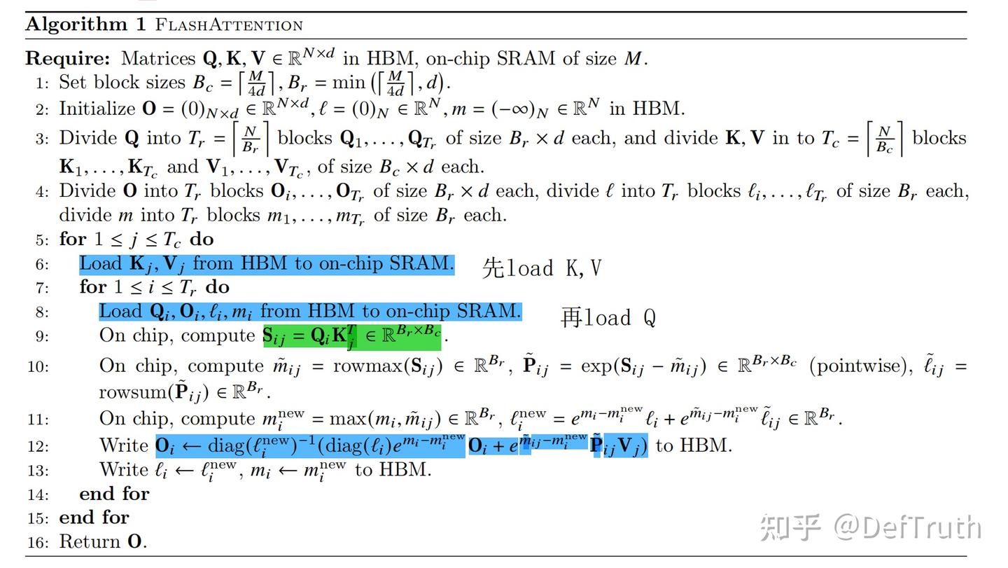
因为 $$\tilde{\mathbf{P}}{ij} = e^{\mathbf{S}{ij}-\tilde{m}{ij}}$$$$e^{\tilde{m}{ij}-m_i^{new}}\tilde{\mathbf{P}}{ij} = e^{\tilde{m}{ij}-m_i^{new}}e^{\mathbf{S}{ij}-\tilde{m}{ij}} = e^{\mathbf{S}_{ij}-m_i^{new}} $$

Backward Pass

前向计算流程如下，计算出 Attention $O$ 之后，继续前向传播得到损失 $L$。 $$ \begin{aligned} S &= QK^T \ P &= softmax(S) \ O &= PV \ L &= f(O) \ \end{aligned} $$ 反向时，假设已知 $\frac{\partial{L}}{\partial{O}}$，记做 $dO \in R^{N\times d}$ ，目标是求得 $\frac{\partial{L}}{\partial{Q}},\frac{\partial{L}}{\partial{K}},\frac{\partial{L}}{\partial{V}}$，即 $dQ, dK, dV \in R^{N\times d}$

$$ \begin{aligned} dV &= \frac{\partial{L}}{\partial{V}} = \frac{\partial{L}}{\partial{O}} \frac{\partial{O}}{\partial{V}} = P^T dO \ dP &= \frac{\partial{L}}{\partial{P}} = \frac{\partial{L}}{\partial{O}} \frac{\partial{O}}{\partial{P}} = dO V^T \ dS &= \frac{\partial{L}}{\partial{S}} = \frac{\partial{L}}{\partial{P}} \frac{\partial{P}}{\partial{S}} = dP \frac{\partial{P}}{\partial{S}} \ dQ &= \frac{\partial{L}}{\partial{Q}} = \frac{\partial{L}}{\partial{S}} \frac{\partial{S}}{\partial{Q}} = dS K \ dK &= \frac{\partial{L}}{\partial{K}} = \frac{\partial{L}}{\partial{S}} \frac{\partial{S}}{\partial{K}} = dS^T Q \ \end{aligned} $$ 其中 P 为 softmax (S)，经过 softmax 中的求导推导，可以得出

$$ dS_{ij} = P_{ij}\left( dP_{ij} - \sum_l P_{il}dP_{il} \right) $$

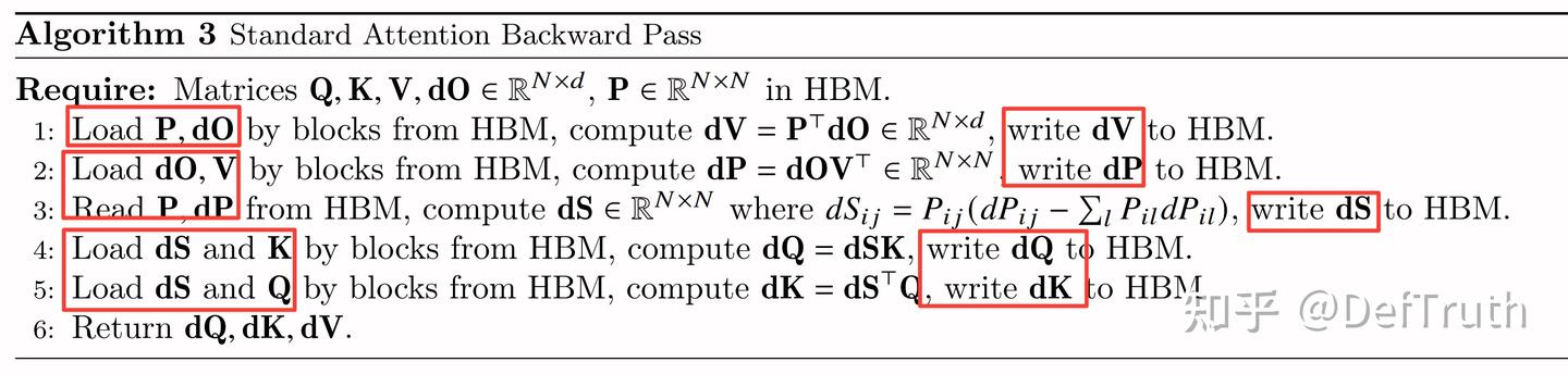
标准 Attention backward pass 计算如下：

对于 FlashAttention 的 backward 计算流程如下

• 参考： https://zhuanlan.zhihu.com/p/669926191

  

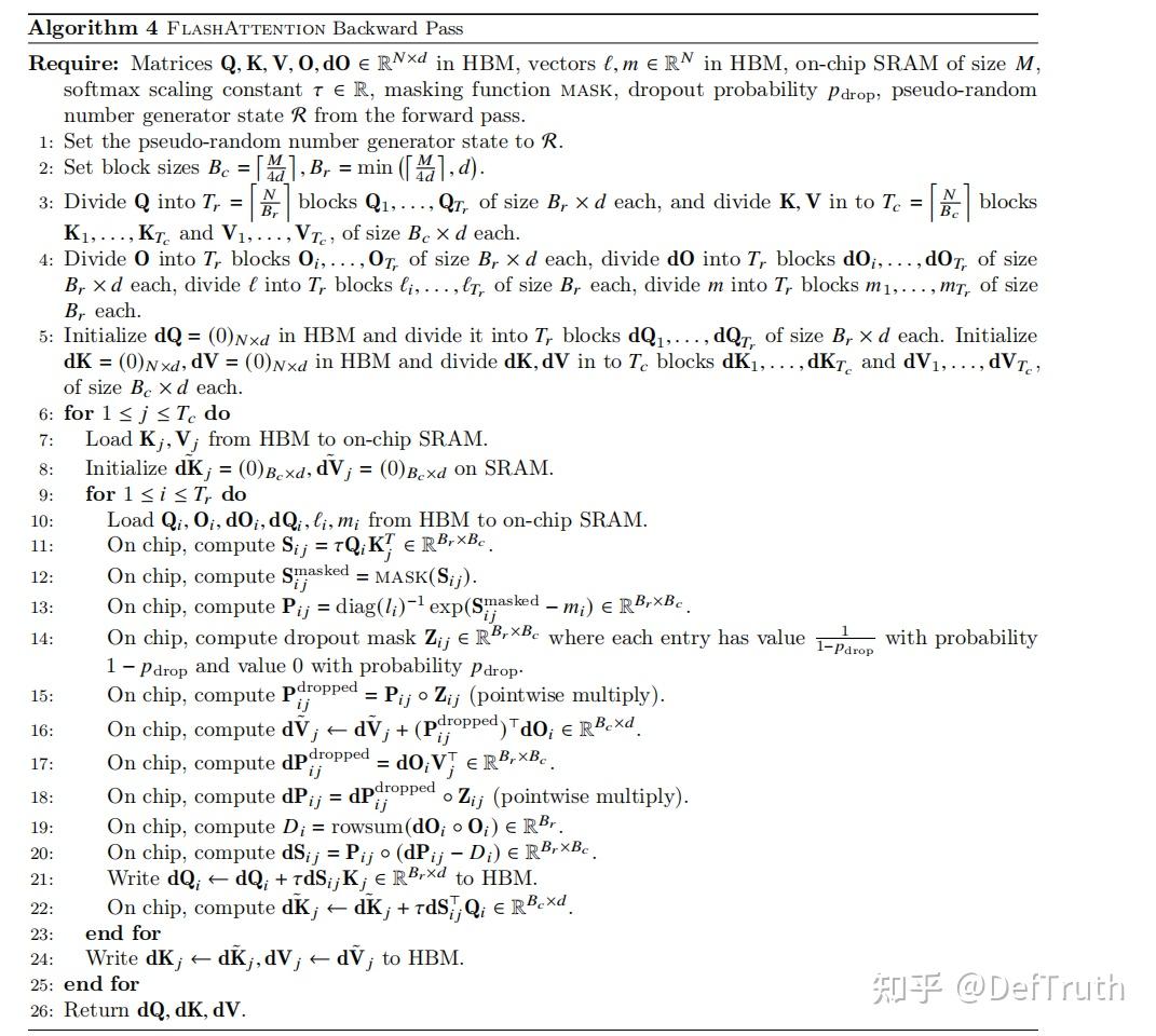
FlashAttention backward pass 最主要的优化就是：Recompute。对比 Standard Self Attention，FlashAttention 在前向不需要保留 S 和 P 矩阵，但是 backward pass 又需要 S 和 P 矩阵的值来计算梯度。那么怎么办呢？那自然就是就是和 forward 一样，利用 Tiling 技术，将 Q, K, V 分块 load 到 SRAM，然后通过 online recompute 计算得到当前块的 S 和 P 值。具体到 backward pass 中计算逻辑就是：

那么，这样做带来的优化是什么呢？首先，针对 Q,K,V 矩阵，无论是否有 recompute，都是必须要 load 到 SRAM 进行计算的，因为计算梯度需要。那么，没有 recompute 时，P 矩阵是事先算好保存在 HBM 中的，此时在 backward 时，需要 load Q,K,V,dO,dS + load P,dP + write dS,dP,dQ,dV,dK。

在使用了 recompute+tiling 后，则只需要 load Q,K,V,dO + write dQ,dV,dK，这个公式可能没有算的很精确，但总的意思就是关于 S,P,dS,dP 的 load/write IO 被消除了。虽然 recompute 增加了计算量 FLOPs，但是 IO 的减少带来的收益更大。按照 NV PTX ISA 8.1 6.6章节-Operand Costs 中的文档说明，GPU HBM IO Accesses 通常耗时>100 时钟周期，而计算指令一般只需要几个时钟周期。

Flash Attention v2

FlashAttention-2 相对于 FlashAttention-1，进一步改变了 Tiling 的顺序，将 Q 矩阵的循环挪到了最外层，这样就可以将 Q 矩阵的循环交给 Thread Block 来并行计算。也就是说，除了原来 batch 和 head 两个维度可以并行，现在也可以在 sequence 维度切分，三层循环分给不同的 thread block，进一步增加 GPU 的吞吐。

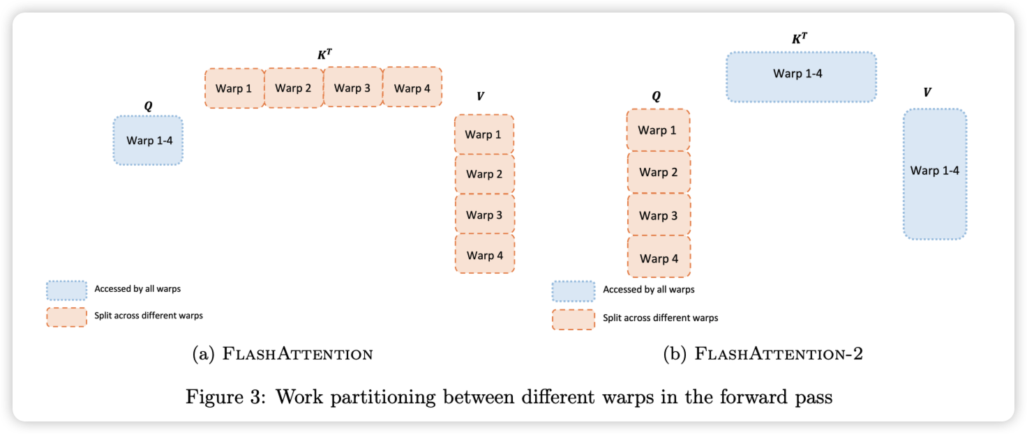
循环顺序调换之后，进一步的对同一个 block 中的 warp patition 做了优化，将 V1 版本中沿着 K 切共享 Q 变成 V2 中沿着 Q 切共享 K。每个 warp 执行矩阵乘法以获得 $QK^T$ 的切片，然后只需与 V 的共享切片相乘就能获得相应的输出切片。Warp 之间不需要通信，共享内存读写的减少也可以提升速度。

Forward Pass

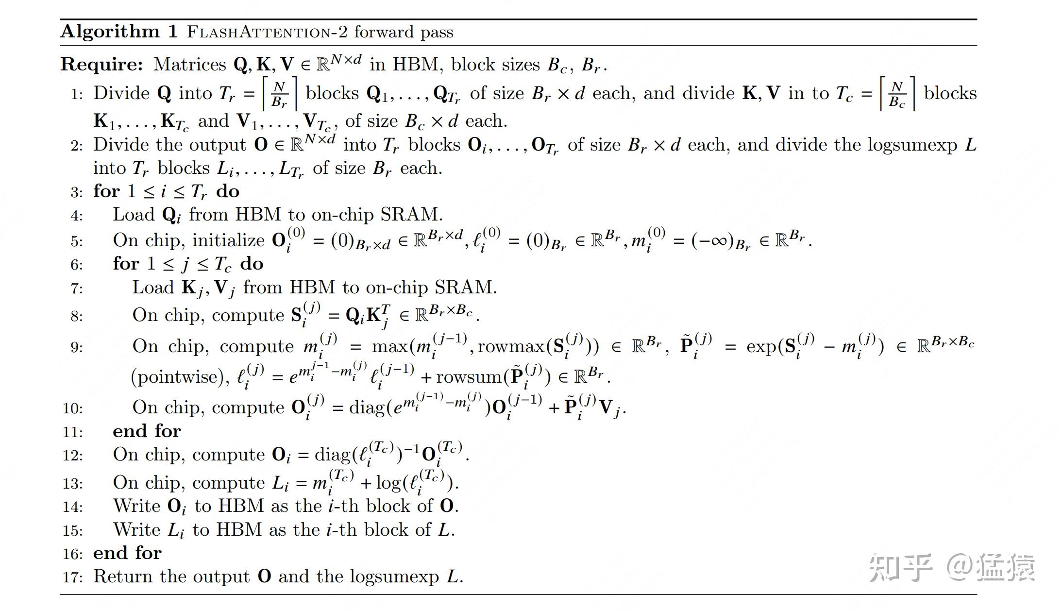
比起 V1，V2中不用再存每一 Q 分块对应的 $m_i$ 和 $l_i$ 了。但是在 BWD 的过程中，我们仍需要 $m_i, l_i$ 来做 $S_i^{(j)}$ 和 $P_i^{(j)}$ 的重计算，这样才能用链式求导法则把 dQ，dK，dV 正常算出来。

V2在这里用了一个很巧妙的方法，它只存一个东西（代码13行，这样又能进一步减少 shared memory 的读写）：$L_i = m_i^{(T_c)} + log(l_i^{(T_c)})$，这个等式中小写的 m 和 l 可以理解成是全局的 rowmax 和 rowsum。在接下来 BWD 的讲解中，我们会来看到这一项的妙用。

Backward Pass

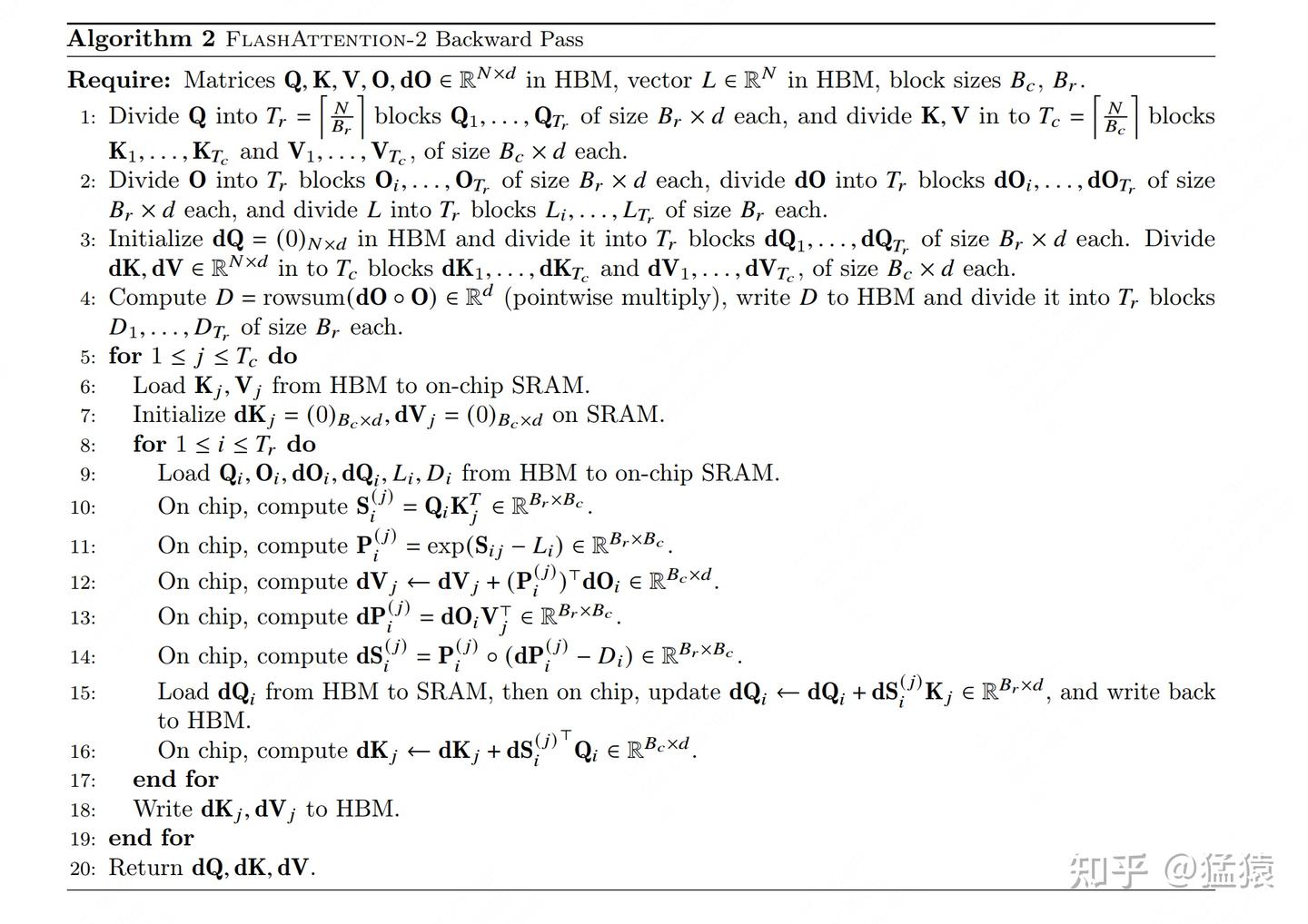
我们知道在BWD的过程中，我们主要是求$dV_j, dK_j, dQ_i$（为了求它们还需要求中间结果$dS_{ij}, dP_{ij}$），我们来总结一下这些梯度都需要沿着哪些方向AllReduce：

• $dV_j$：沿着$i$方向做AllReduce，也就是需要每行的结果加总
• $dK_j$：沿着$i$方向做AllReduce，也就是需要每行的结果加总
• $dQ_i$：沿着$j$方向做AllReduce，也就是需要每列的结果加总
• $dS_{ij}, dP_{ij}$：只与当前$ij$相关

基于此，如果你还是保持Q外循环，KV外循环不变的话，这种操作其实是固定行，遍历列的，那么在这些梯度中，只有$dQ_i$从中受益了，K和V的梯度则进入了别扭的循环（也意味着要往shared memory上写更多的中间结果）；但如果你采用KV外循环，Q内循环，这样K和V都受益，只有Q独自别扭，因此是一种更好的选择。（S和P的计算不受循环变动影响）。

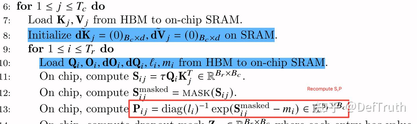
前面说过，在BWD过程中读写我们要用全局的$m_i^{(j)}, l_i^{(j)}$重新计算$P_i^{(j)}$，计算公式如下：

$$P_i^{(j)} = diag(l_i^{(j)})^{-1}exp(S_i^{(j)} - m_i^{(j)})$$

但如此一来，我们就要从shared memory上同时读取$m_i^{(j)}, l_i^{(j)}$，似乎有点消耗读写。所以在V2中，我们只存储$L_i = m_i^{(j)} + log(l_i^{(j)})$，然后计算：

$$P_i^{(j)} = exp(S_i^{(j)} - L_i)$$

很容易发现这两个计算是等价的，但V2的做法节省了读写量

参考

• https://courses.cs.washington.edu/courses/cse599m/23sp/notes/flashattn.pdf