Diffusion Model 的数学推导

前置数学知识

贝叶斯定理

Bayes' theorem ² $$ P(A \mid B) = \frac{P(A)P(B \mid A)}{P(B)} $$

高斯分布

高斯分布 Gaussian distribution ³ 也称作正态分布 Normal distribution，如果随机变量 $X$ 服从一个平均数为 $\mu$ ，标准差为 $\sigma$ 的正态分布，记为： $$ X \sim \mathcal{N}(\mu,\sigma^{2}) $$ 其概率密度函数为： $$ f(x) = \frac{1}{\sigma \sqrt{2\pi}} e^{-\frac{(x-\mu)^2}{2\sigma^2}} $$

当 $\mu = 1$，$\sigma =0$ 时，则称作标准正态分布 。

高斯混合模型

一个复杂的概率分布 $P (x)$ ，可以由多个高斯分布来表示，这即是高斯混合模型。高斯混合模型 Gaussian Mixture Model 是由多个高斯分布组成的模型，起概率密度函数位多个高斯概率密度函数的加权组合，即：

$$ P(x) = \sum_{i=1}^K P(z_i)P(x|z_i) = \sum_{i=1}^k w_i \mathcal{N}(x|\mu_i,\sigma_i^{2}) $$ 其中 $w_i$ 为第 $i$ 个高斯分布的权重系数，并满足 $$ w_i \geq 0, \sum_{i=1}^K w_i = 1 $$

因此，假设我们要求一个复杂的概率分布 $P (x)$ ，只要我们知道了对于 $k$ 个高斯分布，其每一个 $w_m, \mu_m, \sigma_m$ ，就求解出来了这里的 $P (x)$ 。

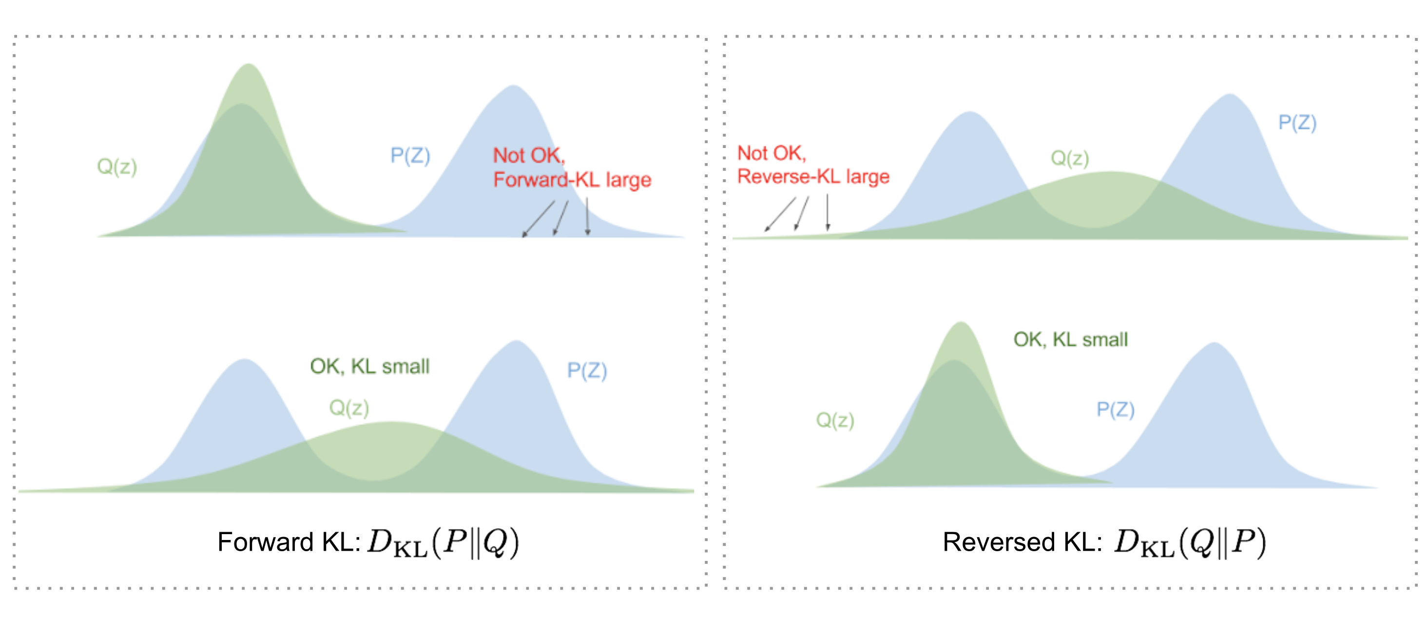
KL 散度

KL 散度 Kullback-Leibler Divergence ⁴ ，又称相对熵 relative entropy，是两个概率分布 $p$ 和 $q$ 差别的非对称性的度量

$$ \begin{align} D_{KL}(p||q) &= \sum_i^m p(x_i)log\frac{p(x_i)}{q(x_i)} \ &= -\sum_i^m p(x_i)log\frac{q(x_i)}{p(x_i)} \ &= - \intop_x p(x)log\frac{q(x)}{p(x)}dx (m \to \infty) \end{align} $$ 一般情况下，$P$ 表示数据的真实分布，$Q$ 表示数据的理论分布、估计的模型分布、或 $P$ 的近似分布。

KL 散度具有以下特性：

• 正定性： $D_{KL}(P||Q) \ge 0$
• 不对称性：$D_{KL}(P||Q) \ne D_{KL}(Q||P)$

从统计学上看，KL 散度可以用来衡量两个分布之间的差异程度。若二者差异越小，则 KL 散度越小，否则反之越大。当两分布一致时，其 KL 散度为 0。正是因为其可以衡量两个分布之间的差异，所以在 VAE、EM、GAN、Diffusion 模型中均有使用到 KL 散度。

对于两个单一变量的高斯分布 $p$ 和 $q$，其中 $p \sim \mathcal{N}(\mu_1,,\sigma_1^{2})$， $q \sim \mathcal{N}(\mu_2,,\sigma_2^{2})$，则他们的 KL 散度为： $$ D_KL(p||q) = log\frac{\sigma_2}{\sigma_1} + \frac{\sigma_1^2 + (\mu_1-\mu_2)^2}{2\sigma_2^2} - \frac{1}{2} $$

Jensen 不等式

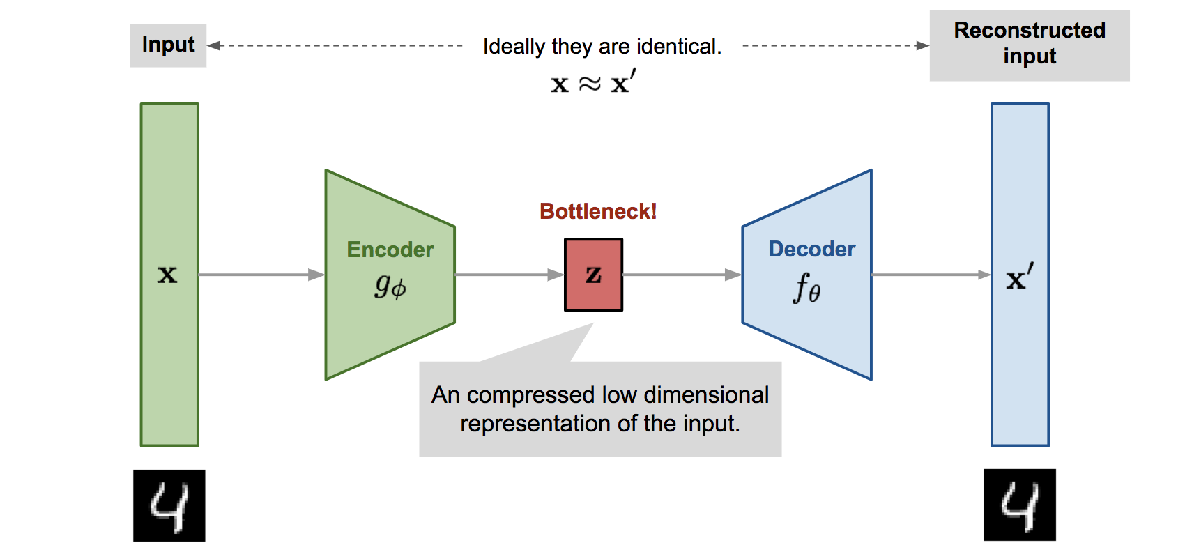
AutoEncoder

• Encoder network
• Decoder network

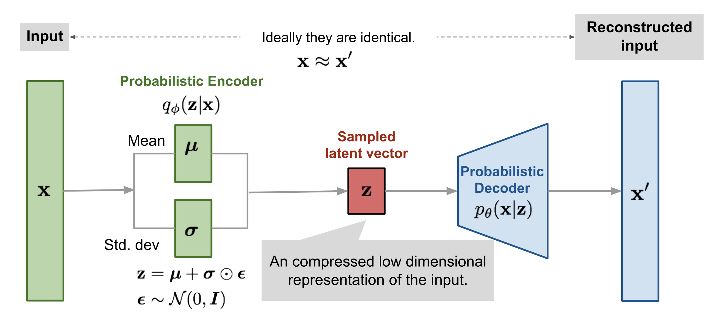
VAE

以李宏毅老师课程中的 Pokemon 样本为例，每一个 Pokemon 图 (h,w,c) 都可以定义成高维空间中的一个点，真实的数据样本在高维空间中存在着对应的概率分布 $P_{data} (x)$ 。

== 图

只要我们有一个模型，无论是 VAE 模型还是 Diffusion 模型，只要它预测的概率分布 $P_{\theta}(x)$ 能够和真实概率分布 $P _{data}(x)$ 尽可能近，那么我们随机从这个模型中采样，那么采样得到的样本就会和真实样本概率就会很大。比如从 Pokemon 数据集中训练出来的模型，sample 得到的样本会长得像 Pokemon。

按照高斯混合模型，我们用多个高斯分布去模拟真实样本的数据分布 $P_{data}(x)$ 。问题是这里的 $k$ 该取多少呢？不同高斯分布对应的比例 $P (z_i)$ 又如何表示呢？

我们用一个连续的标准高斯分布 $P (z)$ 来表示 $P (z_i)$，即 $P (z) \sim \mathcal{N}(1,0)$，则： $$ P_{\theta}(x) = \int P(z) P_{\theta}(x|z) $$

DDPM

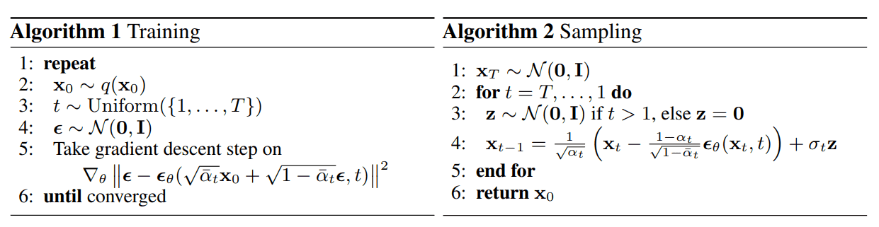
DDPM¹ 的本质是通过模型学习训练数据的分布，产出尽可能符合训练数据分布的真实图片。

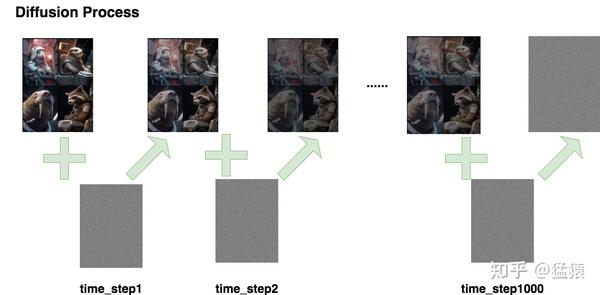
• Diffusion Process，即 Forward Process，这个过程就是一步一步的加噪声

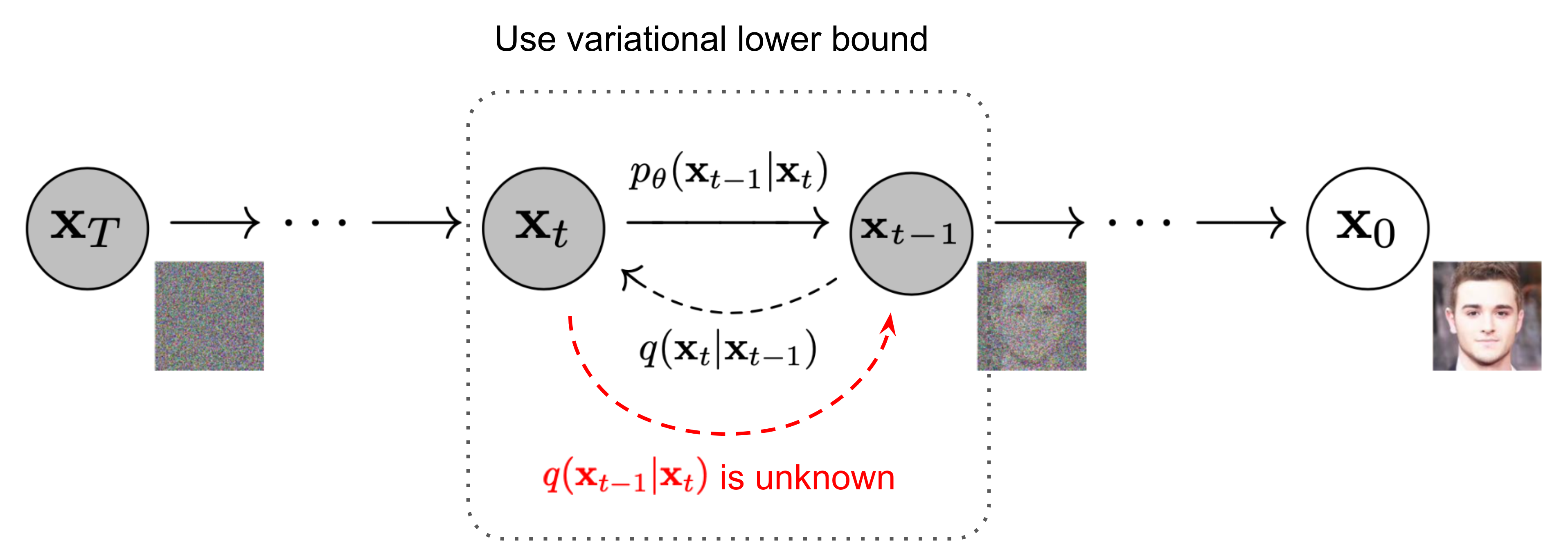
• Denoise Process，即 Reverse Process，这个过程是一步一步的去噪

• https://zhuanlan.zhihu.com/p/530602852

设置符号：

• $T$ ：总步数
• $\mathbf{x_0}, \mathbf{x_1}, …, \mathbf{x_T}$ ：每一步产生的图片，其中 $\mathbf{x_0}$ 是原始图片，$\mathbf{x_T}$ 为纯高斯噪声
• $\epsilon \sim \mathcal{N}(0,,1)$ ：为每一步添加的高斯噪声
• $q(\mathbf{x_t} \mid \mathbf{x_{t-1}})$ ：$\mathbf{x_t}$ 在条件 $\mathbf{x} = \mathbf{x_{t-1}}$ 下的概率分布，代表 diffusion process
• $p(\mathbf{x_{t-1}} \mid \mathbf{x_{t}})$ ：$\mathbf{x_{t-1}}$ 在条件 $\mathbf{x} = \mathbf{x_t}$ 下的概率分布，代表 denoise process。

Diffusion Process

给定初始数据分布 $\mathbf{x_0} \sim q(\mathbf{x})$ ，我们定义一个前向扩散过程 forward diffusion process：

• 我们向数据分布中逐步添加高斯噪声，加噪过程持续 $T$ 次，产生一系列带噪声图片 $\mathbf{x_0}, \mathbf{x_1}, …, \mathbf{x_T}$
• 在由 $\mathbf{x_{𝑡−1}}$ 加噪到 $\mathbf{x_t}$  的过程中，噪声的标准差/方差是以一个在区间 $(0,1)$ 内的固定值 $\beta_t$ 来确定的，均值是以固定值 $\beta_t$  和当前时刻的图片数据 $\mathbf{x_{t-1}}$ 来确定的。

因此，根据以上流程

$$ \mathbf{x_t} = \mathbf{x_{t-1}} + \epsilon_{t-1} = \mathbf{x_0} + \epsilon_0 + \epsilon_1 + … + \epsilon $$

对于最后一步： $$ \mathbf{x_T} = \mathbf{x_{T-1}} + \epsilon_{T-1} = \mathbf{x_0} + \epsilon_0 + \epsilon_1 + … + \epsilon_{T-1} $$

其中：

$$ q (\mathbf{x_t} \mid \mathbf{x_{t-1}}) = \mathcal{N}(\mathbf{x_t}; \sqrt{1-\beta_t} \mathbf{x_{t-1}}, \beta_t \mathbf{I}) $$

$$ q(\mathbf{x_{1:T}} \mid \mathbf{x_0}) = \prod_{t=1}^T q (\mathbf{x_t} \mid \mathbf{x_{t-1}}) $$

上式意思是：

• 由​ $\mathbf{x_{t−1}}$  得到​ ​ $\mathbf{x_t}$  的过程 ​ $𝑞(\mathbf{x_t}|\mathbf{x_{t−1}})$ ，满足分布​  $\mathcal{N}(\mathbf{x_t}; \sqrt{1-\beta_t} \mathbf{x_{t-1}}, \beta_t \mathbf{I})$
• 这个分布是指以​ $\sqrt{1-\beta_t} \mathbf{x_{t-1}}$ 为均值，$​\beta_t$ 为方差的高斯分布
• 我们看到这个噪声只由​ $\beta_t$ 和 ​ $\mathbf{x_{t−1}}$ 来确定，是一个固定值而不是一个可学习过程
• 因此，只要我们有了​ $\mathbf{x_0}$ ，并且提前确定每一步的固定值，$\beta_1, \beta_2, …, \beta_T$ ​，我们就可以推出任意一步的加噪数据 $\mathbf{x_1}, …, \mathbf{x_t}$ ​
• 这里 Forward 加噪过程是一个马尔科夫链过程

随着​ $t$ 的不断增大，最终原始数据​ $\mathbf{x_0}$ 会逐步失去它的特征。最终当 $T \to \infty$ ​时， $\mathbf{x_t}$ ​趋近于一个各向独立的高斯分布。从视觉上来看，就是将原本一张完好的照片加噪很多步后，图片几乎变成了一张完全是噪声的图片。

重参数

在逐步加噪的过程中，我们其实并不需要一步一步地从 $\mathbf{x_0}, \mathbf{x_1},…$ 去迭代得到 $\mathbf{x_t}$ 。事实上，我们可以直接从 $\mathbf{x_0}$ 和固定值序列 ${{\beta_T \in (0, 1)}}_{t=1}^T$ 直接计算得到。

根据重参数技巧，我们可以一步推理出 $\mathbf{x_t}$，计算方法如下所示：

$$ \mathbf{x_t} = \sqrt{\bar{\alpha_t}} \mathbf{x_0} + \sqrt{1-\bar{\alpha_t}} \epsilon $$

推导过程为：

设置 $\alpha_t = 1 - \beta_t$ 以及 $\bar{\alpha_t} = \prod_{i=1}^t \alpha_i$

根据由​ $\mathbf{x_{t−1}}$  得到​ ​ $\mathbf{x_t}$  的过程 ​ $q(\mathbf{x_t}|\mathbf{x_{t−1}})$ ，满足分布​  $\mathcal{N}(\mathbf{x_t}; \sqrt{1-\beta_t} \mathbf{x_{t-1}}, \beta_t \mathbf{I})$，有

$$ \mathbf{x_t} = \sqrt{1-\beta_t} \mathbf{x_{t-1}} + \beta_t \epsilon_{t-1} $$ 也就是： $$ \mathbf{x_t} = \sqrt{\alpha_t} \mathbf{x_{t-1}} + \sqrt{1-\alpha_t} \epsilon_{t-1} $$ 其中 $\epsilon_{t-1}, \epsilon_{t-2},… \sim \mathcal{N}(0,1)$ 为每一步添加的高斯噪声，进一步推导：

总结一下 diffusion process 过程中的公式：

一般地，我们随着​ $t$ 的增大，数据越接近随机的高斯分布， $\beta_t$ ​的取值的取值就越大。所以 $\beta_1 < \beta_2 < \dots < \beta_T$ ，同样的，$\bar{\alpha}_1 > \dots > \bar{\alpha}_T$ 。

Denoise Process

这里 $C(\mathbf{x_t}, \mathbf{x_0})$ 是一个关于 $\mathbf{x_t}$ 和 $\mathbf{x_0}$ ​，而不包含 $\mathbf{x_{t-1}}$ ​的函数，这里省去了具体细节。根据高斯分布的概率密度，这里的方差和均值可以分别写成：

根据 diffusion process 中推导的 $\mathbf{x_t}$ 和 $\mathbf{x_0}$ ​的关系，我们有 $$ \mathbf{x}_0 = \frac{1}{\sqrt{\bar{\alpha}_t}}(\mathbf{x}_t - \sqrt{1 - \bar{\alpha}_t}\boldsymbol{\epsilon}_t) $$ 代入上式则有：

总结下 denoise process 过程中的公式

优化目标

DDPM 的目标就是使得生成的图片尽可能符合训练数据的分布。

通过推导，优化目标从最开始的 令模型输出的分布逼近真实图片的分布 转变为 $argmax_{\theta} \prod_{i=1}^m P_{\theta}(x_i)$，也就是说，要使得连乘中的每一项最大，也等同于使得 $logP_{\theta}(x)$ 最大。

DDIM

Classifier Guidance

Classifier-free Guidance

Model Architecture

U-Net

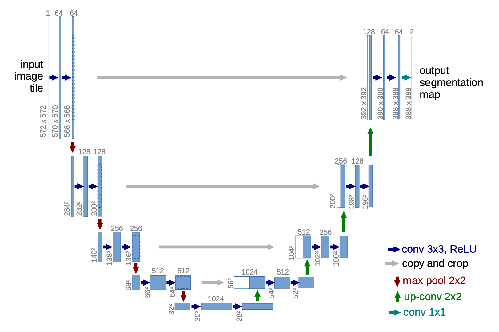
DownSampling

UpSampling

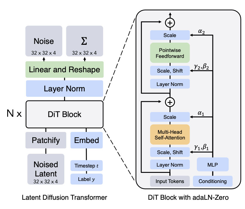
DiT

 1
 2
 3
 4
 5
 6
 7
 8
 9
10
11
12
13
14
15
16

    def forward(self, x, t, y):
        """
        Forward pass of DiT.
        x: (N, C, H, W) tensor of spatial inputs (images or latent representations of images)
        t: (N,) tensor of diffusion timesteps
        y: (N,) tensor of class labels
        """
        x = self.x_embedder(x) + self.pos_embed  # (N, T, D), where T = H * W / patch_size ** 2
        t = self.t_embedder(t)                   # (N, D)
        y = self.y_embedder(y, self.training)    # (N, D)
        c = t + y                                # (N, D)
        for block in self.blocks:
            x = block(x, c)                      # (N, T, D)
        x = self.final_layer(x, c)                # (N, T, patch_size ** 2 * out_channels)
        x = self.unpatchify(x)                   # (N, out_channels, H, W)
        return x

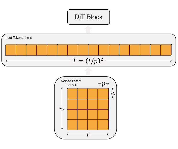
Patchify

输入到 DiT 的 tensor 已经是 noise latent，对应

input batch: N
input size: H, W
in channels: C
patch size: p

也就是 input 的 tensor shape 为 (N, H, W, C) 比如 (N, 32, 32, 4) 。经过 PatchEmbed，输出一系列的 Tokens，对应 token 的 shape 为：

• sequence length: T = (H * W) / (p * p) = 32*32/(2*2)=256
• each patch dim: patch_dim = p * p * C
• 通过 MLP 将 patch 映射 D 大小的维度，patch embedding (T, D)

 1
 2
 3
 4
 5
 6
 7
 8
 9
10
11
12
13
14
15
16
17
18
19
20
21

class PatchEmbed(nn.Module):
    """ Image to Patch Embedding
    """
    def __init__(self, img_size=224, patch_size=16, in_chans=3, embed_dim=768):
        super().__init__()
        img_size = to_2tuple(img_size)
        patch_size = to_2tuple(patch_size)
        num_patches = (img_size[1] // patch_size[1]) * (img_size[0] // patch_size[0])
        self.img_size = img_size
        self.patch_size = patch_size
        self.num_patches = num_patches

        self.proj = nn.Conv2d(in_chans, embed_dim, kernel_size=patch_size, stride=patch_size)

    def forward(self, x):
        B, C, H, W = x.shape
        # FIXME look at relaxing size constraints
        assert H == self.img_size[0] and W == self.img_size[1], \
            f"Input image size ({H}*{W}) doesn't match model ({self.img_size[0]}*{self.img_size[1]})."
        x = self.proj(x).flatten(2).transpose(1, 2)
        return x

DiTBlock

 1
 2
 3
 4
 5
 6
 7
 8
 9
10
11
12
13
14
15
16
17
18
19
20
21
22

class DiTBlock(nn.Module):
    """
    A DiT block with adaptive layer norm zero (adaLN-Zero) conditioning.
    """
    def __init__(self, hidden_size, num_heads, mlp_ratio=4.0, **block_kwargs):
        super().__init__()
        self.norm1 = nn.LayerNorm(hidden_size, elementwise_affine=False, eps=1e-6)
        self.attn = Attention(hidden_size, num_heads=num_heads, qkv_bias=True, **block_kwargs)
        self.norm2 = nn.LayerNorm(hidden_size, elementwise_affine=False, eps=1e-6)
        mlp_hidden_dim = int(hidden_size * mlp_ratio)
        approx_gelu = lambda: nn.GELU(approximate="tanh")
        self.mlp = Mlp(in_features=hidden_size, hidden_features=mlp_hidden_dim, act_layer=approx_gelu, drop=0)
        self.adaLN_modulation = nn.Sequential(
            nn.SiLU(),
            nn.Linear(hidden_size, 6 * hidden_size, bias=True)
        )

    def forward(self, x, c):
        shift_msa, scale_msa, gate_msa, shift_mlp, scale_mlp, gate_mlp = self.adaLN_modulation(c).chunk(6, dim=1)
        x = x + gate_msa.unsqueeze(1) * self.attn(modulate(self.norm1(x), shift_msa, scale_msa))
        x = x + gate_mlp.unsqueeze(1) * self.mlp(modulate(self.norm2(x), shift_mlp, scale_mlp))
        return x

U-Net: Convolutional Networks for Biomedical Image Segmentation, https://arxiv.org/pdf/1505.04597 https://huggingface.co/blog/annotated-diffusion